PYTHON · ML · CLOUD · Commercial property portfolio, 62 buildings
GridWatch IllustrativeAnomaly Detection on Building Energy Telemetry
Every one of 1,480 half-hourly meters across a 62-building commercial portfolio was recording, and nothing was reading them. A fault surfaced when a quarterly bill looked high — typically 60 to 90 days after a chiller had started running through the night. I built unsupervised anomaly detection on the telemetry that raises a ranked, costed alert to the facilities team within hours.
This is an anonymised, illustrative scenario — representative of the shape of engagement and the way I work, not a named client or a delivered set of results. The real, named work on this site is labelled as such.
- €318k annualised energy waste identified across the portfolio
- 4.2 h median detection time, from 60+ days
- 1,480 half-hourly meters monitored continuously
Value returned
€318k
Annualised energy waste identified
Across a portfolio of 62 buildings, ranked by euros per day so the queue is worked in cost order.
Time returned
4.2h
Median time to detect an anomaly
From a baseline of 60-plus days, when a fault surfaced only in a quarterly bill review.
Effort invested
13 weeks
Effort to build
Consulting data scientist — detection design, deployment and facilities-management handover.
Quality
68%
Alert precision
Up from 21% at launch, once cause codes from closed alerts fed back into the model.

01 — Context
The problem.
Half-hourly data existed for every meter and was effectively unread. With 1,480 series there was no realistic way for a facilities team to eyeball them, and the few thresholds someone had configured were static — so they fired constantly in January and never in June. Most alerts were ignored, which is the normal end state for an alert nobody trusts.
The failures being missed were mundane and expensive: schedules left on after a bank holiday, a stuck valve, simultaneous heating and cooling, a chiller cycling all night in an empty building.
02 — Method
The approach.
The build, in the order it happened.
-
A baseline per meter, not per portfolio
Each meter gets its own expected profile from a seasonal-trend decomposition conditioned on day type, occupancy schedule and heating and cooling degree days. Anomaly means departure from that meter’s own expectation, which is the only definition that survives a portfolio this varied.
-
Two detectors, deliberately different
A residual-based statistical detector catches sustained level shifts; an isolation forest over shape features catches profile changes that leave the daily total unchanged — the overnight-running case that a total-consumption check misses entirely.
-
Ranked by euros, not by z-score
Every alert carries an estimated cost per day using the site’s actual tariff and standing charges. The facilities team works a list ordered by money, which is what made them work the list at all.
-
Closed the loop on outcomes
Each alert is closed with a cause code by the engineer who attended. Those codes tune the detectors and, after ten weeks, let false positives be suppressed by pattern rather than by raising a global threshold.
03 — Outcome
What changed.
- Median detection time fell from over 60 days to 4.2 hours from the onset of an anomaly.
- €318k of annualised waste identified in the first two quarters, of which €241k was remediated within the period.
- Alert precision improved from 21% at launch to 68% by week twelve as cause codes fed back into the detectors.
- The single largest find was a chiller running unoccupied overnight in one building for an estimated 11 weeks, at roughly €640 a week.
04 — Before & after
The same measures, either side of the work.
Each pair is scaled against its own larger value, so the comparison is honest rather than flattering.
Median time to detect an energy anomaly
−99.7%- Before
- 1512 hours
- After
- 4.2 hours
Alert precision
+223.8%- Before
- 21 %
- After
- 68 %
Meters monitored continuously
new- Before
- 0 meters
- After
- 1480 meters
05 — The numbers
Median time to detect an energy anomaly.
Tracked as hours, from Baseline through Wk 14 — low 4.2, high 1512.
06 — Screens
What it looks like in use.
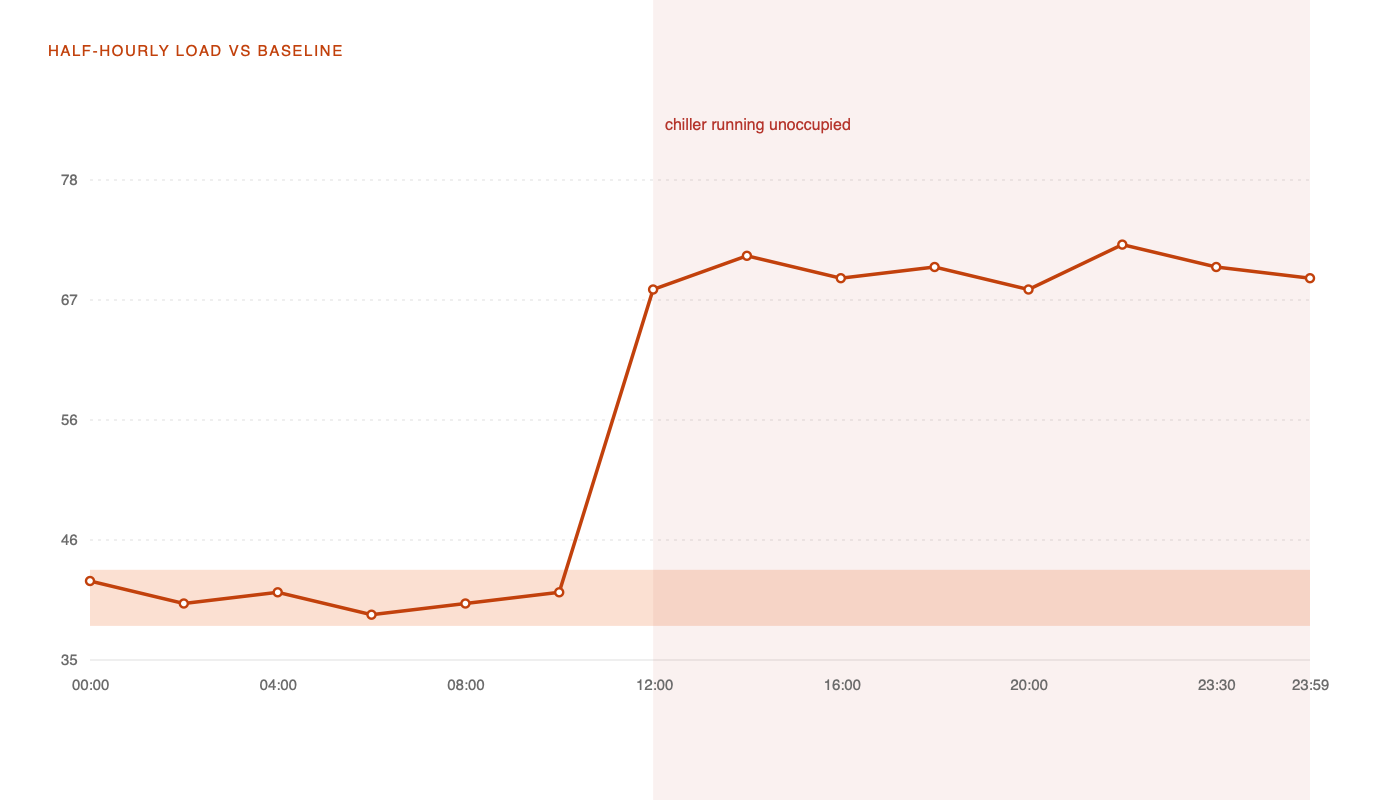
One meter against its own baseline. The overnight shoulder is the chiller — invisible in the daily total, obvious in the profile.
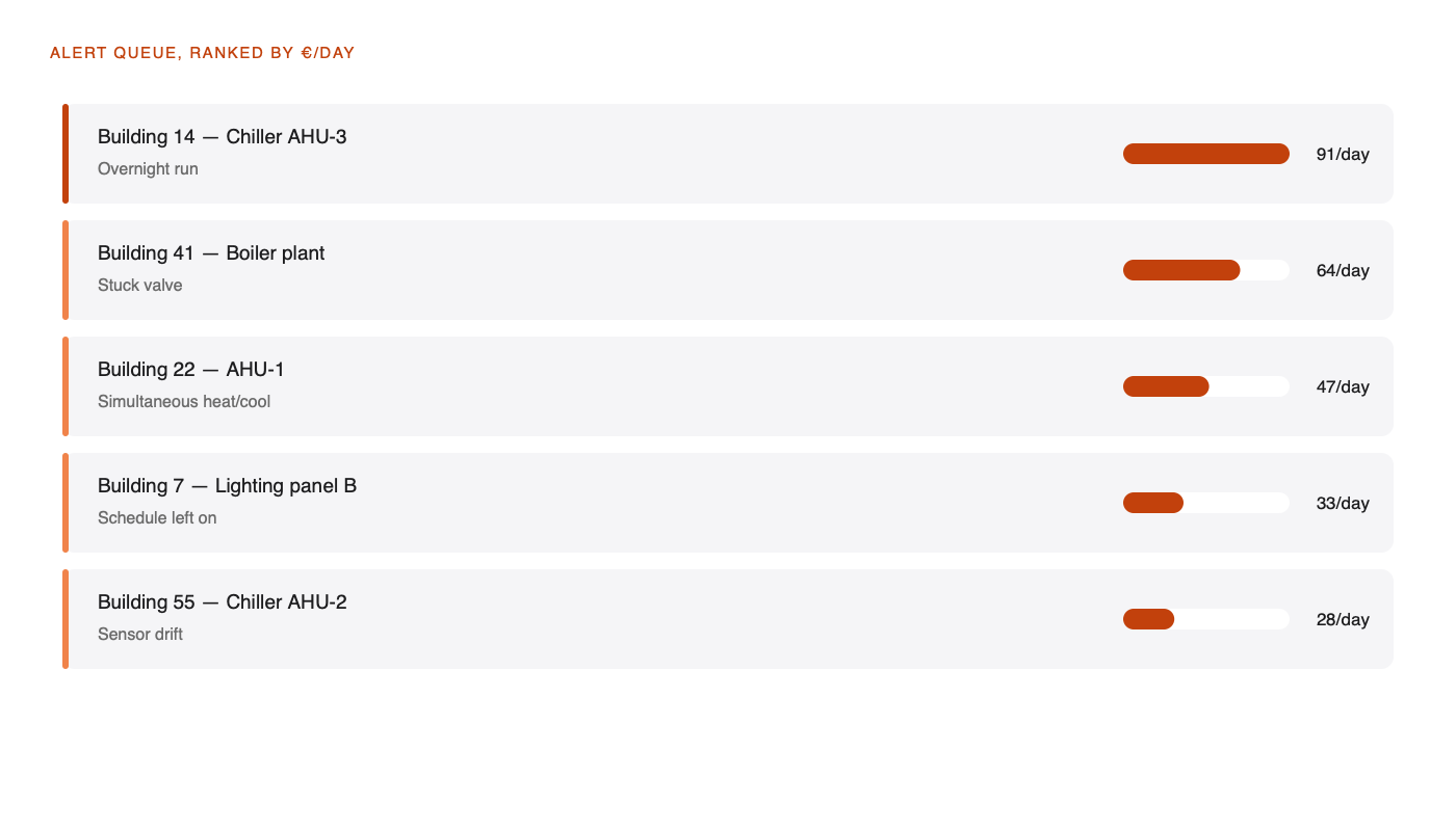
The alert queue, ordered by euros per day. Cause codes from closed alerts are what lifted precision from 21% to 68%.
07 — Stack & role
Built with.
- Python (Pandas, scikit-learn, statsmodels)
- BigQuery
- Cloud Functions
- SQL
- Looker Studio
- Role
- Consulting data scientist — detection design, deployment, FM handover
- Duration
- 13 weeks
- Client
- Commercial property portfolio, 62 buildings
- Period
- 2026
08 — Questions
The questions I get asked about this one.
There were no labelled faults to train on — that was the whole problem. Unsupervised detection plus engineer-supplied cause codes bootstraps the labels, and a supervised layer becomes viable once enough have accumulated.
Heating and cooling degree days are covariates in each meter’s baseline, so a cold snap raises the expectation instead of raising 1,480 alerts.
Ranking by cost and closing every alert with a cause code. An alert with a euro figure attached gets attended; a z-score does not.